import pandas as pdPandas è una libreria python per manipolare ed analizzare dati.
Viene usato per salvare, manipolare, visualizzare dati multidimensionali ed eterogenei. È compatibile con ndarrays.
Strutture dati in pandas
Series
- tipo colonna di uno spreadsheet
- contiene valori e indici
- i valori sono contenuti in una ndarray
- gli indici non devono essere per forza unici, ma l’unicità velocizza molto ed è assunta implicita spesso
Una Serie è una array unidimensionale omogenea
# prende ndarray o python arrays
s1 = pd.Series([1,2,3,4,5])
s1.index.name = Animal
s.name = legs

pd.Series([1,2,3,4], index=[2,3,4,5])
Ha due colonne: una è per l’indicizzazione e una per i dati.
Series properties
s1 = pd.Series([1, 2, 3, 4, 5])
s1.values
# array([1, 2, 3, 4, 5])
s1.array
# <NumpyExtensionArray>
# [np.int64(1), np.int64(2), np.int64(3), np.int64(4), np.int64(5)]
# Length: 5, dtype: int64
s1.index
# RangeIndex(start=0, stop=5, step=1)
s1.dtype
# dtype('int64')
s1.shape
# (5,)
Data selection
Ogni elemento può essere indirizzato sia attraverso label sia attraverso posizione.
s.loc['Paris']
# oppure
s.iloc[2]
s.iloc[1:3] # valori con indice da 1 a 2 compreso
DataFrame
- tipo spreadsheet o SQL table
- collezione di serie che condividono un indice
# From a dictionary of lists
data = {'Name': ['John', 'Anna', 'Peter', 'Linda'],
	'Age': [28, 34, 29, 42],
	'City': ['New York', 'Paris', 'Berlin', 'London']}
df = pd.DataFrame(data)

print(df)
# Name Age City
# 0 John 28 New York
# 1 Anna 34 Paris
# 2 Peter 29 Berlin
# 3 Linda 42 London


data = {'city': ['Bangalore', 'Bangalore', 'Bangalore',
	'Mumbai', 'Mumbai', 'Mumbai'],
	'year': [2020, 2021, 2022, 2020, 2021, 2022,],
	'population': [10.0, 10.1, 10.2, 5.2, 5.3, 5.5]}
# we can specify the columns order
df2 = pd.DataFrame(data, columns=['year', 'city', 'population'])
print(df2)
# outputs:
# year city population
# 0 2020 Bangalore 10.0
# 1 2021 Bangalore 10.1
# 2 2022 Bangalore 10.2
# 3 2020 Mumbai 5.2
# 4 2021 Mumbai 5.3
# 5 2022 Mumbai 5.5- axis=1 freccia a destra
- axis=0 freccia verso il basso
Import and export
# Reading data
df = pd.read_csv('file.csv') # CSV files
df = pd.read_excel('file.xlsx') # Excel files
df = pd.read_json('file.json') # JSON files
df = pd.read_sql('query', connection) # SQL databases

# Writing data
df.to_csv('output.csv') # CSV files
df.to_excel('output.xlsx') # Excel files
df.to_json('output.json') # JSON files
df.to_sql('table_name', connection) # SQL databases
Esplorazione dei dati
df.head() # First 5 rows
df.tail() # Last 5 rows
df.info() # DataFrame information
df.describe() # Statistical summary
df.shape # Dimensions (rows, columns)
df.columns # Column names
df.dtypes # Data types of each column
df.isnull().sum() # Count of missing values
Visualizzazione dei dati
df1 = pd.DataFrame()
df1['A'] = pd.Series(list(range(100)))
df1['B'] = np.random.randn(100, 1)
# plot it
df1.plot(x='A', y='B')
plt.show()

# For instance, we can plot a bar graph out of 4 series:
df2 = pd.DataFrame(np.random.rand(10, 4),
columns=['A', 'B', 'C', 'D'])
df2.plot.bar()
Grafici:
- .plot.barh()
- .plot.barh(stacked = True)
- .plot.hist(stacked = True, alpha=0.7)
- .plot.hist(stacked=True,alpha=0.7,bins=20)
- .plot.box()
- .plot.area()
- .plot.area(stacked=False)
- .plot.scatter(‘A’,‘B’)
Data selection
df['Artist']
df[1:3]
df.loc[1:3,['Artist']]

# loc necessita della label
# df.loc[row_label, column_label]
# iloc è basato su interi
# df.iloc[row_index, column_index]
Data Filtering
# Simple conditions
df[df['Age'] > 30]
df[df['City'] == 'New York'] # Age greater than 30
# City is New York

# Multiple conditions
df[(df['Age'] > 30) & (df['City'] == 'New York')] # AND
df[(df['Age'] > 30) | (df['City'] == 'New York')] # OR

# Other filters
df[df['Name'].isin(['John', 'Anna'])] # Values in a list
df[df['City'].str.contains('New')] # String contains
Missing Values
df.dropna() # rimuove righe della tabella che hanno valori mancantiRaggruppamento
df.groupby('Genre').sum()

# Group by one column
df.groupby('City').mean()
df.groupby('City').count()
df.groupby('City').size() # Mean of numeric columns per city
# Count of values per city
# Size of each group

# Group by multiple columns
df.groupby(['City', 'Gender']).mean()

# Custom aggregations
df.groupby('City').agg({'Age': 'mean', 'Salary': ['min', 'max']})
df.groupby('City').agg({'Age': ['min', 'max', 'mean', 'count']})
Data Transformation
# Adding new columns
df['DoubleAge'] = df['Age'] * 2
df['FullName'] = df['FirstName'] + ' ' + df['LastName']

# Applying functions
df['Age'].apply(lambda x: x * 2) # Using lambda
df['Name'].apply(len) # Getting string lengths

# Transforming values
df['City'] = df['City'].str.upper() # Convert to uppercase
df['Code'] = df['Code'].astype(str) # Change data type

# creare colonna con colonne già esistenti
df['Avg plays'] = df['Plays']/df['Listeners']
Arithmetic operations
In mixed operations between DataFrames and Series, the Series is treated like a row vector and aligned accordingly.
Merging and joining
# Merge DataFrames (SQL-like join)
pd.merge(df1, df2, on='ID')
pd.merge(df1, df2, on='ID', how='left')
pd.merge(df1, df2, on='ID', how='right')
pd.merge(df1, df2, on='ID', how='outer') # Inner join
# Left join
# Right join
# Outer join
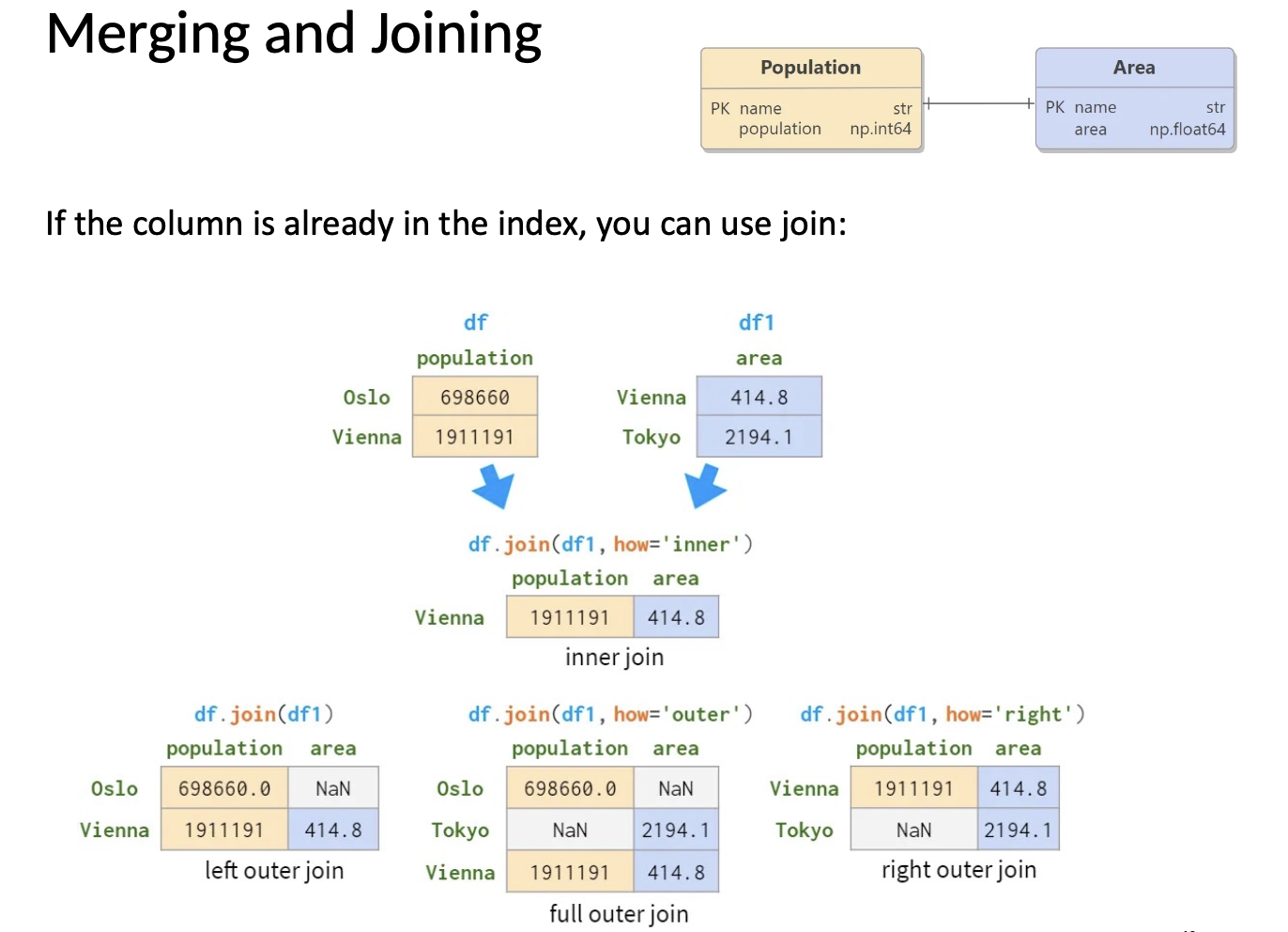
# Join using indexes
df1.join(df2) # Join on index
# Concatenate DataFrames
pd.concat([df1, df2]) # Stack vertically
pd.concat([df1, df2], axis=1) # Stack horizontally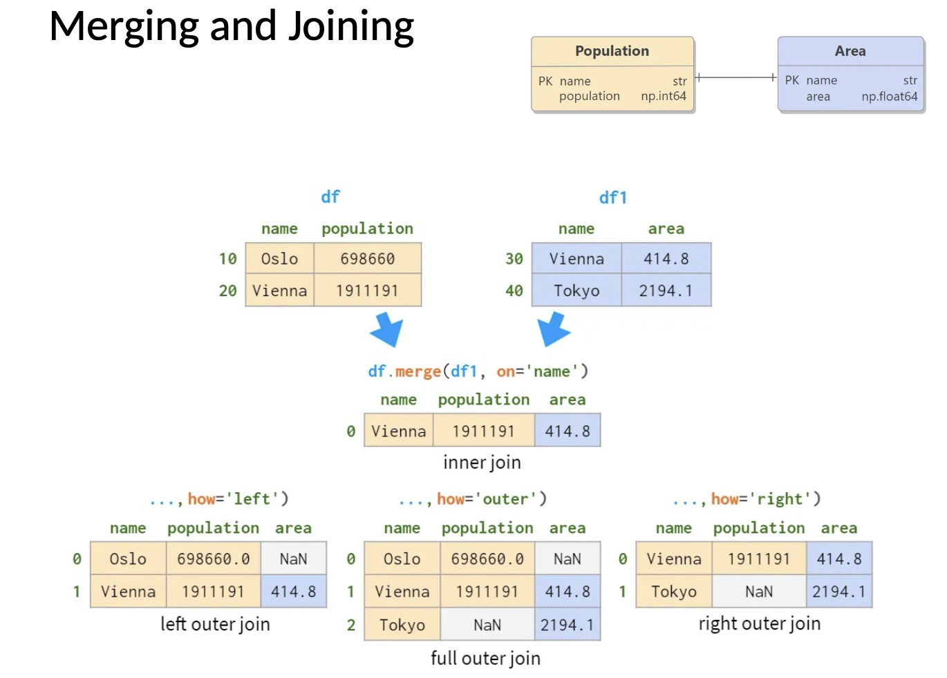
Data reshaping
# Pivot tables
df.pivot_table(index='City', columns='Gender', values='Salary', aggfunc='mean')

# Melt (unpivot) - convert from wide to long format
pd.melt(df, id_vars=['ID'], value_vars=['Score1', 'Score2'],
	var_name='Exam', value_name='Score')

# Stack and unstack
df.stack() df.unstack() # Pivot from columns to index
# Pivot from index to columns
Time series analysis
# Creating date ranges
dates = pd.date_range(start='2023-01-01', end='2023-01-10')
dates = pd.date_range(start='2023-01-01', periods=10, freq='D')

# Time-based indexing
df['Date'] = pd.to_datetime(df['Date']) # Convert to datetime
df.set_index('Date', inplace=True) # Set date as index
df['2023-01'] # Select by month
df['2023-01-01':'2023-01-05'] # Select date range

# Time-based resampling
df.resample('M').mean() # Monthly average
df.resample('W').sum() # Weekly sum
Performance
Optimize your Pandas code for better performance:
• Use vectorized operations instead of loops
• Use .loc and .iloc for faster indexing
• Filter data early to reduce the size of your dataset
• Use appropriate data types to reduce memory usage
• Consider using pandas.read_csv() with usecols to load only needed
columns
• For large datasets, consider chunking with chunksize parameter
• Use inplace=True when appropriate to avoid copies