Image Processing with PyTorch

uni

from torchvision import transforms
 
# Define a transformation pipeline
transform = transforms.Compose([
	transforms.Resize((224, 224)),
	transforms.ToTensor(), # Convert to tensor and normalize to [0,1]
	transforms.Normalize(
		mean=[0.485, 0.456, 0.406], # ImageNet means
		std=[0.229, 0.224, 0.225] # ImageNet standard deviations
	)
])
# Apply transformations to an image
from PIL import Image
img = Image.open('image.jpg')
img_tensor = transform(img) # Shape: [3, 224, 224]

Traditional Patter recognition models use hand-crafted features and relatively simple trainable classifiers.

Deep Learning: implemented as a composition of non-linear transformations of the data with the goal of learning features directly from data.
We can first extract features from an image and then apply the trainable classifier to the output features.

CNNs

But MLPs/deep convolutional neural networks do not scale well: every neuron must be connected to every input pixel.
This is why we use convolutional filters: CNNs only connect each neuron to only a local region of the input volume. The spatial extent of this connectivity is a hyper-parameter called the receptive field of the neuron (equivalently this is the filter size). It is implicitly assumed that statistics is similar at different
locations.

In CNNs a node receives only a small set of features which are spatially close to each other (e.g. 3x3, 5x5) called receptive field from one layer to the next.

The key characteristics of the Convolutional layer are local connectivity and weight sharing.

Complete CNN architecture

Typically CNNs are are composed of a cascade of:

• Convolutional-ReLu layers: perform convolution over the input and non-linear transform over the convolution output
• Spatial pooling layers: output a summary statistics of local input
• Fully-connected ReLu layers (one or several): perform combination of final convolutional outputs

Layers of a CNN have neurons arranged in 3 dimensions (width, height, depth). Each layer of a ConvNet transforms one volume of activations to another through a differentiable function.

A Softmax classifier is used to perform final classification CNNs are trained by supervised learning: i.e. the convolutional filters are trained by back‐propagating the classification error.

1. input
2. convolution (learned)
3. non-linearity
4. spatial pooling
5. fully connected
6. non-linearity
7. softmax

1 - Convolution

A convolutional layer of a CNN is just like a filter, but its parameters are learned.

The output of a convolutional layer is called a feature map.

Sobel filters (filters that extract edges: $\left[\begin{array}{ccc}-1& 0& 1\\ -1& 0& 1\\ -1& 0& 1\end{array}\right]$) convolved with an image extracts a feature map.

Feature Map size

The size of a feature map is given by 3 hyperparameters, decided before the convolution step is performed:

• zero-padding: how many zeros we pas around the border of the feature map
• stride: how much we slide the filter
• depth: number of filters to use (kernel size)

output size:

$$O=\frac{InputSize-FilterSize+2(zeroPadding)}{stride}+1$$

Alex Krizhevsky wrote the first paper about CNNs.

2 - Non-linearity

3 - Spatial Pooling

Spatial Pooling partitions the input image into a set of non-overlapping rectangles and, for each such sub-region, outputs the maximum / average value of the features in that region.
Max-pooling or average-pooling: choosing the maximum or the average as final ouput of the sub-region.

Reduces the spatial size of the representation to reduce the amount of parameters and computation in the network and hence to also control overfitting.

Pooling layers provide invariance to small transformations and reduce the effect of noises and shift or distortion.

Today pooling is not performed anymore, we just play with the stride: in such a way that the windows overlap.

Different CNN architectures

Let’s see some CNN architectures currently used for computer vision tasks.

CNNs are typically composed of 2 parts:

• feature extraction
• classification

The input data at each layer is an image. With each layer we are applying a new convolution over a new image. Each image is a 3D object that has a height, width, and depth. Depth is referred to as the color channel where depth = 1 for grayscale images and 3 for color images.
In the later layers, the images still have depth but they are not colors per se.
They are feature maps that represent the features extracted from the previous layers.

Typically, either all fully-connected layers in a network have the same number of hidden units or decrease at each layer.
Research has found that keeping the number of units constant doesn’t hurt the neural network so it may be a good approach if you want to limit the number of choices you have to make when designing your network.
Pick a number of units per layer and apply that to all your FC layers.

LeNet-5

AlexNet

Dataset: imageNet

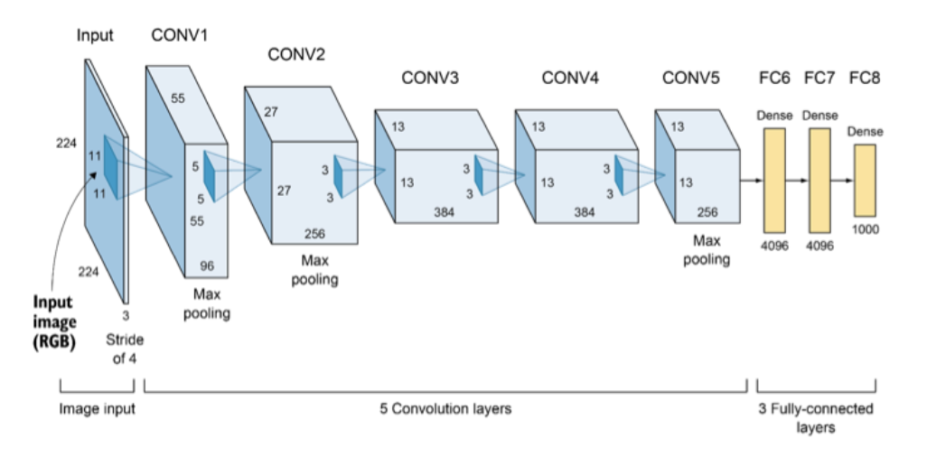
From LeNet it :

• introduces ReLu
• uses a dropout layer: during training at every different image a different half of final neurons is disabled, this is done to make sure no neuron relies on other neurons.
• uses weight regularization
• uses data augmentation: creating new images from training using transformations like flipping, scaling, rotation ecc.
• uses local response normalization

VGGNet

Developed by Oxford in 2014, available in two versions: VGG16 and VGG19: 16 vs 19 convolutional weight layers.

Structure: 2/3 convolutional layers and then pooling, and repeat.

Inception/GoogLeNet

By Google, 2014, much less parameters but more layers.

Not stacked architecture: it introduces inception modules, which do parallel operations: different convolutional layers take as input the same image/features, and give different features which then get concatenated.

They also introduced fully connected layers also in the middle of the pipeline, to counter translation after translation during the pipeline and getting a more stable training. This introduces auxiliary loss, computed during training and ignored during inference (the optimization becomes multi-target - Pappalardo hates to see this simple trick).

ResNet

Microsoft, 2015.

Introduces Skip connections. This enabled many more layers possible. The model with skip connections doesn’t slowly loose track anymore, it gains ancho points in the middle of the pipeline.

Transfer Learning

Transfer learning uses pre-trained models on large datasets as starting points.

• requires less training data
• faster-training
• better performace

Popular pre-trained models:

• ResNet
• VGG
• MobileNet
• EfficientNet
• YOLO (for object detection)

model = models.resnet18(pretrained=True) # oppure False se vogliamo allenarlo noi
 
# Freeze layers
for param in model.parameters():
	param.requires_grad = False
# THIS BECOMES A FEATURE EXTRACTOR
	
# replace final layer for new task, eg with 5 classes
num_features = model.fc.in_features
model.fc = nn.Linear(num_feature, 5)
# now only fc layer parameters will be updated during training

Object Detection

Locate and classify multiple objects in an image.

Popular architectures:

• YOLO (you only look once)
• Faster R-CNN
• SSD (single shot detector)
• RetinaNet

Key concepts:

• bounding boxes
• confidence scores
• non-maxim suppression (NMS)
• IoU (intersection over Union)

Regional proposal

These methods propose some zones, and the second phase analyzes these proposed boxes and works on those.

NMS

But a single object can be inside multiple bounding objects.

As the name implies, NMS technique looks at all the boxes surrounding an object to find the box that has the maximum prediction probabilities and suppress or eliminate the other boxes.

Hyperparams: probability threshold, IoU threshold

Detection Metrics

$$\text{IoU (intersection over Union)}=\frac{\text{Area of Overlap}}{\text{Area of Union}}$$

• FPS for detection speed
• mAP for network precision (mean Average Precision)